Machine learning for public health doesn’t require a PhD. You need working knowledge of three core paradigms (supervised, unsupervised, reinforcement learning), when to use logistic regression versus gradient boosting, how to avoid overfitting, and why feature engineering with domain expertise beats algorithm sophistication for most problems.
Learning Objectives
This chapter provides working knowledge of machine learning fundamentals. You will learn to:
Distinguish three ML paradigms (supervised, unsupervised, reinforcement learning)
Select appropriate algorithms based on problem structure and interpretability needs
Recognize overfitting, data leakage, and bias-variance tradeoff
The Big Picture:You don’t need a PhD in machine learning, you need enough knowledge to choose the right tool, avoid catastrophic mistakes, and communicate with technical teams. This chapter provides working knowledge of ML fundamentals focused on practical public health applications.
Three ML Paradigms (Pick the Right One):
Supervised Learning (most common in public health AI): Learn from labeled examples (input + correct output) → predict outcomes. Use when you have historical data with known answers (disease diagnosis, outbreak prediction, risk stratification)
Unsupervised Learning: Find hidden patterns in unlabeled data (clustering, anomaly detection). Use for exploratory analysis and discovering structure
Reinforcement Learning: Learn optimal actions through trial and error. Sounds cool but much harder than supervised learning, only use for sequential decision optimization
Algorithm Selection Guide (Start Simple, Add Complexity Only If Needed):
Logistic Regression: Your default starting point. Interpretable coefficients (odds ratios), works with modest data, fast, epidemiologists understand it intuitively
Random Forests: Best first “real” ML model. Robust, handles messy data, provides feature importance, works out-of-the-box
Gradient Boosting (XGBoost): Maximum accuracy for tabular data. Consistently outperforms neural networks on structured data, but more hyperparameters to tune
Deep Learning: Only for images (CNNs), text (transformers), or truly complex patterns. For tabular public health data, trees usually win
Critical Reality Check: For most public health spreadsheet data (rows and columns), gradient boosting beats neural networks. Save deep learning for medical imaging, clinical notes, and multimodal data.
Evaluation Metrics (Accuracy Alone Is Misleading):
Accuracy: Total correct predictions. Fails with imbalanced data (99% accuracy predicting “no disease” for 1% prevalence = useless)
Sensitivity (Recall): Fraction of actual cases detected. Critical for screening (don’t miss disease)
Specificity: Fraction of healthy correctly identified. Critical when false alarms are costly
ROC-AUC: Gold standard for binary classification. 0.5 = random, 0.7 = decent, 0.8 = good, 0.9 = excellent (check for overfitting!)
Always report confusion matrix so readers can calculate their preferred metric
The Cardinal Sins (What Kills Models):
Overfitting:Training accuracy 95%, test accuracy 65% → model memorized noise. Fix: more data, regularization, simpler model, cross-validation
Data Leakage: Test information contaminates training (e.g., normalizing before splitting). Makes model look better than it is. Always split first, then preprocess
Ignoring Class Imbalance: Rare events (1% outbreaks) need special handling, use class weights, SMOTE, or appropriate metrics (F1, ROC-AUC, not accuracy)
Temporal Violations: For time series, never use future to predict past. Use temporal train/test splits, not random shuffling
The Bias-Variance Tradeoff:
Underfitting (high bias): Model too simple, fails even on training data
Overfitting (high variance): Model too complex, memorizes training data, fails on new data
Sweet spot:Complex enough to capture patterns, simple enough to generalize
The Most Important Lesson:Feature engineering (domain expertise) > algorithm sophistication. A public health analyst who knows which variables matter epidemiologically will beat a computer scientist with fancy algorithms and no domain knowledge. Epidemiologists have an advantage over pure data scientists, use it.
The Takeaway for Public Health Practitioners: Start with logistic regression. Try Random Forests if you need better performance. Use gradient boosting for maximum accuracy on tabular data. Save neural networks for images and text. Always validate on held-out test data. Report multiple metrics. Trust your domain expertise for feature engineering. Most problems don’t need deep learning.
Test your grasp of the key concepts before proceeding:
1. Algorithm Selection: You have a dataset of 5,000 patient records (rows) with 30 clinical variables (columns) predicting hospital readmission. Which algorithm should you try FIRST? - A. Deep neural network with 10 hidden layers - B. Logistic regression - C. Reinforcement learning - D. Large language model
Click for answer
Answer: B. Logistic regression
Why: For tabular public health data with modest size, start simple. Logistic regression is interpretable, works with this data size, and epidemiologists understand it. Save deep learning for images/text or after simpler methods fail.
2. Evaluation Metrics: Your disease screening model has 95% accuracy predicting COVID-19 from symptoms. Disease prevalence is 2%. Should you deploy it? - A. Yes, 95% accuracy is excellent - B. No, need to check sensitivity, specificity, and ROC-AUC first - C. No, accuracy is meaningless for imbalanced data - D. Both B and C
Click for answer
Answer: D. Both B and C
Why: With 2% prevalence, a model predicting “no COVID” for everyone gets 98% accuracy but is useless. For rare events, accuracy is misleading. Must check sensitivity (don’t miss cases), specificity (minimize false alarms), and ROC-AUC.
3. Cardinal Sins: Your model gets 92% training accuracy but only 67% test accuracy. What’s the problem? - A. Data leakage - B. Overfitting - C. Underfitting - D. Class imbalance
Click for answer
Answer: B. Overfitting
Why: Large gap between training and test performance indicates overfitting, model memorized training noise instead of learning generalizable patterns. Fix: more data, regularization, simpler model, cross-validation.
4. Feature Engineering: A data scientist with a PhD in machine learning and a public health epidemiologist with 10 years of field experience are both building outbreak prediction models. Who has the advantage? - A. Data scientist, they know advanced algorithms - B. Epidemiologist, they know which variables matter - C. Neither, both skills are equally important - D. Depends on the problem
Click for answer
Answer: B. Epidemiologist (with a caveat)
Why: Feature engineering (domain expertise) > algorithm sophistication. The epidemiologist knows incubation periods, transmission routes, risk factors, invaluable for creating meaningful features. The data scientist knows tools but not the disease. Best case: collaboration between both.
5. Practical Application: You’re asked to build an AI system to “improve public health.” What should you do FIRST? - A. Choose an algorithm (deep learning is hot right now) - B. Collect as much data as possible - C. Define a specific, measurable problem - D. Read papers on the latest AI techniques
Click for answer
Answer: C. Define a specific, measurable problem
Why: “Improve public health” is too vague. AI solves specific problems: predict hospital readmission, detect disease outbreaks, classify medical images. Start with problem, not technology. Vague goals → failed projects.
Scoring: - 5/5: Excellent! You understand the fundamentals. Ready to proceed. - 3-4/5: Good grasp. Review sections where you missed questions. - 0-2/5: Reread the TL;DR summary above before continuing.
Introduction
You don’t need a PhD in machine learning to use AI effectively in public health. You need to understand just enough to:
Choose the right tool for your problem
Interpret results critically
Avoid common pitfalls
Communicate with technical teams
Know when AI is the wrong solution
This chapter gives you that foundation. We’ll skip the heavy math and focus on concepts, intuition, and practical application.
This chapter provides the working knowledge you need to evaluate AI systems, communicate with technical teams, and make informed decisions about AI adoption.
How Machine Learning Actually Works
Before diving into algorithms, let’s establish what “machine learning” actually means. These concepts underpin everything that follows.
What is a Model?
A model is a mathematical function that maps inputs to outputs. You already use models: logistic regression maps patient characteristics to disease probability. The equation \(\text{logit}(p) = \beta_0 + \beta_1 X_1 + ...\) is a model.
In ML, “model” means the same thing, but models can have millions of adjustable values instead of a handful of \(\beta\) coefficients.
What is “Learning”?
When we say a model “learns,” we mean: the algorithm adjusts numerical values (parameters) to minimize prediction errors on training data.
This is identical to what happens when you fit a logistic regression. The computer finds \(\beta\) values that best predict your outcome. ML extends this to models with vastly more parameters, using different optimization techniques.
What is a Loss Function?
A loss function quantifies how wrong the model’s predictions are. Common examples:
Squared error for regression: \((y_{true} - y_{pred})^2\)
Cross-entropy for classification: measures how far predicted probabilities are from 0/1 truth
Training minimizes this loss. Different problems use different loss functions, and the choice shapes what the model learns to optimize.
What is Gradient Descent?
When you have millions of parameters, you can’t solve for optimal values directly (no closed-form solution). Instead, ML uses gradient descent: an iterative process that finds good parameter values by following the slope of the loss function “downhill.”
Intuition: Imagine finding the lowest point in a valley while blindfolded. You feel which direction goes downhill, take a small step that way, then repeat. Eventually you reach the bottom. That’s gradient descent, the “gradient” tells you which direction is steepest.
The learning rate controls step size: too large and you overshoot; too small and training takes forever.
Parameters vs. Hyperparameters
Two types of numerical values in ML:
Parameters: Learned from data during training (like \(\beta\) coefficients). The model adjusts these automatically.
Hyperparameters: Set by you before training (like tree depth, learning rate, number of hidden layers). These control the learning process itself.
Example: In Random Forest, the number of trees (500) is a hyperparameter you choose. The specific split points in each tree are parameters learned from data.
For Epidemiologists: What You Already Know
Much of ML is familiar under different names:
Biostatistics
Machine Learning
Notes
Predictors, covariates
Features
Identical concept
Outcome, dependent variable
Label, target
Identical concept
Model fitting
Training
Same process, different name
Residual deviance
Loss
Both measure prediction error
LASSO, Ridge regression
Regularization
Identical technique
Validation sample
Test set
Similar purpose
Penalized likelihood
Regularized loss
Same mathematical approach
You already understand the core concepts. ML extends them to larger models and different problem types.
The Three Fundamental Paradigms
All of machine learning falls into three categories, as comprehensively reviewed in Mitchell’s foundational work on machine learning. Master these, and you’ll understand 90% of AI applications in public health.
1. Supervised Learning: Learning from Examples
The Idea: You show the algorithm examples of inputs and correct outputs. It learns the pattern. Then it predicts outputs for new inputs.
Analogy: Teaching a medical student by showing them patient cases with known diagnoses.
Real-world example:
Input: Patient symptoms (fever, cough, chest pain)
Output: Diagnosis (pneumonia)

You show the algorithm 10,000 labeled examples.
It learns: "fever + productive cough + chest pain → pneumonia (85% probability)"
When to use it: - You have labeled historical data (inputs + correct answers) - You want to predict a specific outcome - Examples: disease diagnosis, outbreak prediction, risk stratification
Supervised learning requires labeled data, meaning someone (often human experts) must have already provided the “correct answers” for your training examples.
The Idea: You give the algorithm data with NO labels. It finds structure, patterns, or groups on its own.
Analogy: Sorting a messy pile of patient records into natural categories without being told what categories to use.
Real-world example:
Input: Symptom reports from 50,000 emergency department visits
Output: "I found 7 distinct clusters, one looks like flu-like illness,
   another looks like gastrointestinal illness, etc."
When to use it: - You have unlabeled data (which is most data!) - You want to discover structure or segments - You’re exploring without a specific prediction goal
3. Reinforcement Learning: Learning by Trial and Error
The Idea: An agent takes actions in an environment and receives rewards or penalties. It learns which actions lead to the best outcomes. This approach, formalized by Sutton and Barto in their seminal text, has applications in sequential decision-making.
Analogy: Training a dog, reward good behavior, discourage bad behavior, let it learn through experience.
When to use it: - You’re optimizing sequential decisions - There’s no “correct answer” dataset - You have a simulator or can interact safely
Reinforcement learning sounds exciting but is much harder to implement than supervised learning. It requires careful reward engineering and lots of computational resources.
For most public health problems, supervised learning is more practical. Don’t use RL just because it sounds cool.
For this handbook, we’ll focus primarily on supervised learning. It represents the majority of practical public health AI applications.
Beyond Traditional RL: LLM-Based AI Agents
The “agents” described above refer to traditional reinforcement learning. A newer paradigm has emerged: LLM-based AI agents that combine large language models with tool use (web search, code execution, API calls) to accomplish complex multi-step goals. These agents can plan, act, observe results, and iterate autonomously. For comprehensive coverage of how these agents work, their applications in public health surveillance and epidemiological analysis, and critical safety considerations, see AI Agents: From Chatbot to Autonomous Assistant.
Core Supervised Learning Concepts
The Machine Learning Workflow
Every supervised learning project follows this pattern, as outlined in Geron’s practical guide:
Collect labeled data (features + known outcomes)
Split into train/test sets (typically 80% train, 20% test)
Choose and train a model (algorithm learns patterns from training data)
Evaluate on unseen test data (measure real-world performance)
Deploy and monitor (put into production, track ongoing performance)
Python: ML Workflow Overview
Hide code
# 1. Collect labeled datadata = load_outbreak_data() # Features + outcomes# 2. Split into train/test setstrain_data, test_data = split(data, test_size=0.2)# 3. Choose and train a modelmodel = RandomForestClassifier()model.fit(train_data.features, train_data.outcomes)# 4. Evaluate on unseen test datapredictions = model.predict(test_data.features)accuracy = evaluate(predictions, test_data.outcomes)# 5. Deploy and monitormodel.save('outbreak_predictor.pkl')
Let’s break down each step.
Step 1: Features and Labels
Features (also called “predictors” or “independent variables”): The inputs your model uses to make predictions.
Labels (also called “targets” or “dependent variables”): The outputs you’re trying to predict.
Examples: - Raw: Daily case counts → Engineered: 7-day rolling average - Raw: Birth date → Engineered: Age in years - Raw: GPS coordinates → Engineered: Distance to nearest hospital - Raw: Text symptoms → Engineered: Presence/absence of key symptom terms
This is where epidemiologists have an advantage over pure data scientists. You know which features actually matter biologically and epidemiologically.
Training set (60-70%): Model learns patterns from this
Validation set (10-20%): Used to tune model settings (hyperparameters)
Test set (20%): Never touched until final evaluation, simulates real-world performance
Why this matters:
BAD approach: Tune your model based on test set performance. This “cheats” by peeking at data meant to simulate real-world conditions.
GOOD approach: Use the validation set for all adjustments. Only check the test set once, at the very end.
Python: Train/Validation/Test Splits
Hide code
# BAD: Tuning on test datamodel = train_model(train_data)# Adjust model settings...performance = evaluate(model, test_data) # Too optimistic!# GOOD: Using validation setmodel = train_model(train_data)# Adjust model settings based on validation performance...performance = evaluate(model, validation_data)# Only after all tuning is done:final_performance = evaluate(model, test_data) # True performance
The Cardinal Sin: Data Leakage
Data leakage happens when information from the test set “leaks” into training. This makes your model look better than it really is, a problem extensively documented in Kaufman et al.’s analysis of leakage in healthcare ML.
Common mistakes: - Normalizing features before splitting data - Including future information in features - Using the same patients in both train and test - Cross-validation on time series without respecting temporal order
Machine learning does the same thing, but: - Often with millions of parameters - Using iterative optimization (gradient descent, not closed-form solutions) - With regularization to prevent overfitting - On much larger datasets
The model is literally learning from mistakes: making predictions, measuring how wrong they are (the “loss”), and adjusting parameters to reduce that error. This cycle repeats until performance stops improving.
How Training Works (Technical Detail)
Hide code
# Simplified training loopfor epoch inrange(num_epochs):# Make predictions with current parameters predictions = model.predict(X_train)# Calculate error (loss) error = calculate_loss(predictions, y_train)# Adjust parameters to reduce error gradients = compute_gradients(error) parameters = parameters - learning_rate * gradients# Repeat until error stops decreasing
Common Machine Learning Algorithms
Let’s survey the algorithms you’ll encounter most often in public health AI. For each, we’ll cover how it works, strengths/weaknesses, when to use it, and a practical example.
1. Logistic Regression: Your Old Friend
You already know this one!Logistic regression predicts binary outcomes (disease/no disease, outbreak/no outbreak).
When to use it: - Binary classification problems - You want interpretable coefficients (odds ratios) - You have modest amounts of data - Linear relationships are reasonable
Strengths:
Interpretable (you can explain to stakeholders)
Fast to train
Works well with small data
Provides probability estimates
Epidemiologists understand it intuitively
Weaknesses:
Assumes linear relationships (in log-odds space)
Can’t capture complex interactions automatically
Performance limited on very complex patterns
Python: Logistic Regression
Hide code
from sklearn.linear_model import LogisticRegressionfrom sklearn.metrics import classification_reportimport pandas as pdimport numpy as np# Load outbreak datadata = pd.read_csv('../data/examples/dengue_outbreaks.csv')# Features and labelX = data[['temperature', 'rainfall', 'prev_cases', 'population_density']]y = data['outbreak'] # 0 or 1# Train/test splitfrom sklearn.model_selection import train_test_splitX_train, X_test, y_train, y_test = train_test_split( X, y, test_size=0.2, random_state=42)# Train modelmodel = LogisticRegression(max_iter=1000)model.fit(X_train, y_train)# Evaluatey_pred = model.predict(X_test)print(classification_report(y_test, y_pred))# Interpret: Look at coefficients (like ORs in epi)feature_names = X.columnscoefficients = model.coef_[0]for feature, coef inzip(feature_names, coefficients): odds_ratio = np.exp(coef)print(f"{feature}: OR = {odds_ratio:.2f}")
Output interpretation:
temperature: OR = 1.15 → Each 1°C increase → 15% higher outbreak odds
rainfall: OR = 1.08  → Each 1mm increase → 8% higher outbreak odds
prev_cases: OR = 1.25 → Each additional case → 25% higher outbreak odds
Start Here
Logistic regression should be your default starting point for classification problems. Only move to complex models if it doesn’t work well enough.
Many “AI” successes in public health are just well-applied logistic regression with good feature engineering.
Prediction vs. Inference: A Critical Mindset Shift
In epidemiology, you interpret regression coefficients causally: “Each unit increase in X is associated with Y% higher odds, controlling for confounders.”
In ML, coefficients are prediction weights, not causal effects. A model might weight “time since last outbreak” heavily for prediction even though it’s not causally related to outbreak occurrence. Multicollinearity, which invalidates causal inference, doesn’t hurt prediction.
Key implications:
ML finds correlations, not causes. A model predicting hospital readmission identifies correlated factors, but changing those factors may not reduce readmissions.
Confounding is not automatically addressed. ML may use confounders as predictive features rather than controlling for them.
For causal questions (“Does X cause Y?”), you still need DAGs, propensity scores, instrumental variables, or randomized trials.
If you need to explain why something happens, use epidemiological methods. If you need to predict what will happen, ML often excels.
from sklearn.tree import DecisionTreeClassifierfrom sklearn import treeimport matplotlib.pyplot as plt# Train decision treemodel = DecisionTreeClassifier(max_depth=3, random_state=42)model.fit(X_train, y_train)# Visualize the treeplt.figure(figsize=(20,10))tree.plot_tree(model, feature_names=X.columns, class_names=['No outbreak', 'Outbreak'], filled=True, fontsize=10)plt.savefig('../images/examples/decision_tree.png', dpi=300, bbox_inches='tight')plt.show()# Make predictionspredictions = model.predict(X_test)probabilities = model.predict_proba(X_test)
Strengths:
Highly interpretable (you can draw the exact decision process)
Handles non-linear relationships automatically
No need to normalize features
Works with mixed data types (numerical + categorical)
Can capture interactions between features
Weaknesses:
Prone to overfitting (memorizing training data)
Unstable (small data changes → very different trees)
Often less accurate than ensemble methods
Single trees vs. Forests
Single decision trees are rarely used in production because they overfit easily. Instead, we use ensembles of many trees (Random Forests, Gradient Boosting), see next sections.
But single trees are excellent for exploratory analysis and communicating findings to non-technical stakeholders.
3. Random Forests: Democracy of Trees
The idea: Instead of one decision tree, train hundreds or thousands of trees on slightly different subsets of data. Each tree “votes” on the final prediction. This ensemble method introduced by Breiman (2001) has become one of the most widely used algorithms in machine learning.
Why it works: Individual trees might overfit and make mistakes, but their collective wisdom averages out errors.
Analogy: Instead of asking one doctor, you ask 500 doctors and take the majority opinion.
Python: Random Forests
Hide code
from sklearn.ensemble import RandomForestClassifierfrom sklearn.metrics import roc_auc_score, confusion_matriximport numpy as np# Train random forestmodel = RandomForestClassifier( n_estimators=500, # Number of trees max_depth=10, # Limit tree depth (prevent overfitting) min_samples_split=20, # Require at least 20 samples to split random_state=42)model.fit(X_train, y_train)# Predict probabilities (not just 0/1)y_pred_proba = model.predict_proba(X_test)[:, 1]# Evaluate with ROC-AUCauc = roc_auc_score(y_test, y_pred_proba)print(f"ROC-AUC: {auc:.3f}")# Feature importance: Which features matter most?importances = model.feature_importances_feature_importance_df = pd.DataFrame({'feature': X.columns,'importance': importances}).sort_values('importance', ascending=False)print("\nFeature Importance:")print(feature_importance_df)# Plot with handbook stylingimport syssys.path.append('..')from styles.plot_config import set_handbook_style, HANDBOOK_COLORSset_handbook_style()import seaborn as snsplt.figure(figsize=(10, 6))sns.barplot(data=feature_importance_df, x='importance', y='feature', color=HANDBOOK_COLORS['primary_blue'])plt.title('Feature Importance in Outbreak Prediction')plt.xlabel('Importance Score')plt.tight_layout()plt.savefig('../images/examples/feature_importance.png', dpi=300, bbox_inches='tight')
Strengths:
Very accurate on most problems
Handles thousands of features without feature selection
Resistant to overfitting (unlike single trees)
Provides feature importance scores
No need for feature scaling
Works out-of-the-box with minimal tuning
Weaknesses:
Less interpretable than single trees (500 trees is hard to explain)
Slower to train and predict than simple models
Large file sizes (saving 500 trees takes space)
Can struggle with highly imbalanced data
Practical Advice
Random Forests are often the best first “real” ML model to try after logistic regression. They’re: - Forgiving of mistakes in data preparation - Robust to outliers - Accurate enough for many applications - Easy to use with scikit-learn
For many public health prediction tasks, a well-tuned Random Forest is all you need.
4. Gradient Boosting: The Current Champion
The idea: Build trees sequentially, where each new tree focuses on correcting the mistakes of previous trees. This approach, formalized by Friedman (2001), has become the dominant method for structured data competitions.
Analogy: Instead of 500 doctors voting independently (Random Forest), you have a team of 500 doctors where each successive doctor specifically tries to fix the previous doctor’s misdiagnoses.
Popular implementations: - XGBoost (most popular) - LightGBM (faster, good for large data) - CatBoost (handles categorical features well)
Python: Gradient Boosting (XGBoost)
Hide code
from xgboost import XGBClassifierfrom sklearn.model_selection import cross_val_score# Train XGBoost modelmodel = XGBClassifier( n_estimators=500, learning_rate=0.05, # How much each tree contributes max_depth=6, subsample=0.8, # Use 80% of data for each tree colsample_bytree=0.8, # Use 80% of features for each tree random_state=42)model.fit(X_train, y_train)# Cross-validation for robust performance estimatecv_scores = cross_val_score(model, X_train, y_train, cv=5, scoring='roc_auc')print(f"Cross-validated AUC: {cv_scores.mean():.3f} (+/- {cv_scores.std():.3f})")# Test set performancey_pred_proba = model.predict_proba(X_test)[:, 1]test_auc = roc_auc_score(y_test, y_pred_proba)print(f"Test AUC: {test_auc:.3f}")# Feature importance (SHAP values for better interpretation)import shapexplainer = shap.TreeExplainer(model)shap_values = explainer.shap_values(X_test)# Visualize what drives predictionsshap.summary_plot(shap_values, X_test, feature_names=X.columns)
Strengths:
Often the most accurate “classical” ML algorithm
Consistently outperforms neural networks on tabular data
Handles missing data automatically
Built-in regularization prevents overfitting
Excellent with tabular data (most public health data)
Weaknesses:
More hyperparameters to tune than Random Forests
Easier to overfit if not careful
Requires more computational resources
Even less interpretable than Random Forests (but SHAP values help)
When to Use Gradient Boosting
Use gradient boosting when: - You’ve tried Random Forests and need better performance - You have sufficient data (>10,000 observations) - Prediction accuracy is critical - You have time/resources for hyperparameter tuning
Stick with Random Forests when: - You want simplicity and fast iteration - Data is limited (<1,000 observations) - Interpretability is paramount
5. Neural Networks and Deep Learning
The idea: Layers of interconnected “neurons” that transform inputs into outputs through learned weights. Neural networks are universal approximators, meaning they can theoretically learn any function given enough data and capacity.
Each connection has a “weight” that’s adjusted during training using backpropagation.
When neural networks shine: - Large datasets (millions of examples) - Complex patterns (images, text, audio) - Representation learning (automatic feature extraction)
When they struggle: - Small datasets (<10,000 examples) - Tabular data (trees often work better, as shown in Shwartz-Ziv & Armon 2022) - Interpretability is required
For most public health tabular data (spreadsheets with rows and columns), gradient boosting methods usually outperform neural networks, as demonstrated in multiple systematic comparisons.
Neural networks excel at: - Medical imaging (chest X-rays, histopathology) - Time series with complex temporal patterns - Natural language processing - Multi-modal data (combining images + text + numbers)
For simple prediction from structured data, stick with tree-based methods first.
Deep Learning Architectures for Public Health
Deep learning = neural networks with many layers (10s to 100s of layers), as comprehensively covered in Goodfellow et al.’s textbook.
Key concept: Transfer Learning Instead of training from scratch, start with a model pre-trained on millions of images (ImageNet), then fine-tune it on your medical images. This transfer learning approach works even with small datasets (1,000-10,000 images).
For most public health applications, fine-tuning existing models is more practical than training from scratch.
Quick Algorithm Selection Guide
Use this decision tree to choose algorithms:
Do you have labeled data?
 └─ No → Unsupervised learning (clustering, anomaly detection)
 └─ Yes → Continue...

What type of data?
 └─ Images  → CNNs (ResNet, EfficientNet)
 └─ Text   → Transformers (BERT, GPT)
 └─ Time series → LSTMs, Transformers, or gradient boosting
 └─ Tabular  → Continue...

How much data?
 └─ < 1,000 rows  → Logistic regression, single decision tree
 └─ 1,000-10,000  → Random Forest
 └─ > 10,000   → Gradient boosting (XGBoost)
 └─ > 100,000  → Deep learning (if complex patterns)

Do you need interpretability?
 └─ Critical → Logistic regression or single decision tree
 └─ Nice  → Random Forest + SHAP values
 └─ Less important → Gradient boosting or neural networks
Evaluation Metrics: Measuring Success
You’ve trained a model. How do you know if it’s good?
For Classification (Disease/No Disease, Outbreak/No Outbreak)
Harmonic mean of precision and recall, introduced by van Rijsbergen (1979) in information retrieval. Useful when you need a single metric balancing both.
7. ROC-AUC (Area Under the Receiver Operating Characteristic Curve)
No single metric tells the whole story. The right metric depends on your use case:
Scenario
Primary Metric
Why
Disease screening
Sensitivity
Cannot afford to miss cases
Confirmatory testing
Specificity, PPV
False positives are costly
Balanced classes
F1, Accuracy
Both errors equally important
Imbalanced data
ROC-AUC, PR-AUC
Accuracy is misleading
Rare events (<5%)
Precision-Recall AUC
ROC-AUC can be overoptimistic
Always report the confusion matrix so readers can calculate their preferred metric.
8. Calibration: When Probabilities Must Be Accurate
A model can have excellent discrimination (high AUC) but poorly calibrated probabilities. If your model outputs “70% probability of readmission,” patients with that score should actually be readmitted about 70% of the time.
Why calibration matters in public health:
Clinical decision support: When probability thresholds trigger interventions (e.g., “if risk > 50%, refer to specialist”), the probabilities must be accurate
Cost-benefit analyses: Require accurate probability estimates, not just good ranking
Communicating risk: Telling a patient “you have 80% risk” is only meaningful if 80% is calibrated
How to check calibration:
Reliability diagrams (calibration curves): Plot predicted probabilities vs. observed frequencies. A perfectly calibrated model follows the 45-degree line.
Brier score: Measures both discrimination and calibration; lower is better
A Common Mistake
Many ML practitioners optimize only for AUC and ignore calibration. A model with AUC = 0.90 but poor calibration may be useless for clinical decision-making where you need to trust the probability values, not just the ranking.
For clinical applications, always check calibration using reliability diagrams. See Steyerberg et al. (2010) for calibration assessment in clinical prediction models.
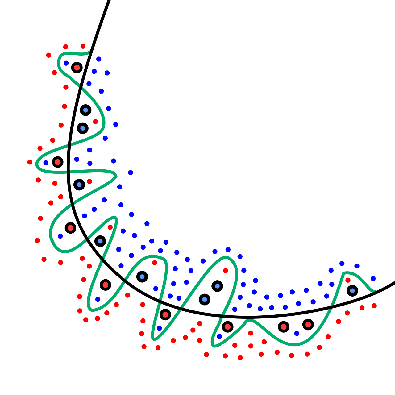
Figure 5.1: Visualization of underfitting vs. overfitting. The green line (left) represents an underfit model that’s too simple to capture the data pattern. The black line (center) shows a well-fit model that generalizes appropriately. The blue curve (right) shows an overfit model that memorizes training data noise and won’t generalize. Source: Wikimedia Commons (Public Domain)
How to Detect Overfitting
Hide code
# Compare training vs. test performancetrain_accuracy = model.score(X_train, y_train)test_accuracy = model.score(X_test, y_test)print(f"Training accuracy: {train_accuracy:.3f}")print(f"Test accuracy: {test_accuracy:.3f}")print(f"Difference: {train_accuracy - test_accuracy:.3f}")
Red flags: - Training accuracy = 0.95, Test accuracy = 0.65 → Overfitting! - Training accuracy = 0.60, Test accuracy = 0.58 → Underfitting (both low) - Training accuracy = 0.82, Test accuracy = 0.80 → Just right (close and good)
How to Prevent Overfitting
More data (the best solution, if possible)
Regularization (penalize model complexity using L1/L2 penalties)
Cross-validation (validate on multiple splits)
Simpler model (fewer features, less depth)
Early stopping (stop training before overfitting starts)
Ensemble methods (average multiple models)
Example with regularization:
Hide code
from sklearn.linear_model import LogisticRegressionCV# CV suffix = automatic cross-validation for hyperparameter tuningmodel = LogisticRegressionCV( Cs=10, # Try 10 different regularization strengths cv=5, # 5-fold cross-validation scoring='roc_auc', random_state=42)model.fit(X_train, y_train)# Best regularization parameter found automaticallyprint(f"Best C (regularization): {model.C_[0]:.4f}")
# BAD: Normalize before splittingfrom sklearn.preprocessing import StandardScalerscaler = StandardScaler()X_scaled = scaler.fit_transform(X) # Uses ALL data including test!X_train, X_test = train_test_split(X_scaled, test_size=0.2)
Correct approach:
Hide code
# GOOD: Split first, then normalizeX_train, X_test = train_test_split(X, test_size=0.2)scaler = StandardScaler()X_train_scaled = scaler.fit_transform(X_train) # Fit on train onlyX_test_scaled = scaler.transform(X_test) # Apply to test
2. Ignoring Class Imbalance
The problem: When one class is rare (e.g., 1% outbreak rate), models can get high accuracy by always predicting the majority class.
Solutions:
Hide code
# Option 1: Use class_weight parametermodel = RandomForestClassifier(class_weight='balanced')# Option 2: Use appropriate evaluation metrics (F1, ROC-AUC, not accuracy)# Option 3: Resample data using SMOTE (Chawla et al., 2002)from imblearn.over_sampling import SMOTEsmote = SMOTE(random_state=42)X_train_balanced, y_train_balanced = smote.fit_resample(X_train, y_train)
The problem: Single train/test split might be lucky or unlucky. Cross-validation, introduced by Stone (1974), provides more robust performance estimates.
Start simple: Logistic regression → Random Forest → Gradient Boosting → Deep Learning. Don’t skip steps.
Feature engineering > Algorithm choice: Domain expertise in creating good features matters more than fancy algorithms.
Evaluation is multi-dimensional: No single metric tells the whole story. Report confusion matrix, ROC-AUC, and metrics relevant to your use case.
Overfitting is the enemy: Always validate on held-out test data. Use cross-validation. Be skeptical of “too good” results.
Interpretability matters: In public health, stakeholders need to understand and trust models. Use SHAP values, feature importance, and simple models when possible.
AI ≠ Magic: It’s pattern recognition from data. Garbage in = garbage out. Your domain knowledge is irreplaceable.
Most problems don’t need deep learning: Trees and ensembles work great for tabular data. Save neural networks for images, text, and truly complex patterns.
Using the outbreak detection code patterns above: 1. Modify features (try removing or adding features) 2. Try different algorithms (logistic regression, decision tree) 3. Compare performance, which works best? Why?
Exercise 2: Handle Imbalance
Create a dataset where outbreaks are only 2% of weeks: 1. Train a model without addressing imbalance 2. Train with class_weight='balanced' 3. Compare using F1 score and ROC-AUC
Exercise 3: Interpret Predictions
Pick one misclassified test example: 1. What features contributed to the wrong prediction? 2. Use SHAP values to visualize 3. Could a human have made the same mistake?
Check Your Understanding
Test your knowledge of machine learning fundamentals and their applications in public health. Each question builds on the key concepts from this chapter.
Question 1
You’re building a model to predict dengue outbreaks using historical data with known outbreak labels (yes/no). You have temperature, rainfall, and previous case counts as features. Which machine learning paradigm should you use?
Unsupervised learning, because weather patterns are complex
Supervised learning, because you have labeled historical outbreak data
Reinforcement learning, because outbreak prediction requires sequential decision-making
Deep learning, because outbreak prediction is a complex task
Correct Answer: b) Supervised learning, because you have labeled historical outbreak data
This is a classic supervised learning problem because:
You have labeled data: Historical weeks with known outbreak outcomes (yes/no)
You have features: Temperature, rainfall, previous case counts
You want to predict a specific outcome: Whether an outbreak will occur
The three fundamental paradigms are distinguished by:
Supervised learning: You have labeled examples (inputs + correct outputs), and you want to predict outcomes for new data
Unsupervised learning: You have unlabeled data and want to discover patterns or structure (clustering, anomaly detection)
Reinforcement learning: You’re optimizing sequential decisions through trial and error with rewards/penalties
Common supervised learning applications in public health include: - Disease diagnosis from symptoms or images - Outbreak prediction from surveillance data - Risk stratification for high-risk patients - Hospital readmission prediction
For this dengue outbreak problem, you’d likely start with logistic regression (binary classification), then try Random Forests or gradient boosting if you need better performance.
Question 2
You’ve trained a model to predict hospital readmissions. Training accuracy is 95%, but test accuracy is only 68%. What is the most likely problem, and what should you do?
Underfitting - use a more complex model with more parameters
Overfitting - the model memorized training data and doesn’t generalize well
Data leakage - information from the test set leaked into training
Class imbalance - readmissions are rare events
Correct Answer: b) Overfitting - the model memorized training data and doesn’t generalize well
The large gap between training (95%) and test (68%) accuracy is a classic sign of overfitting. The model is too complex and has essentially memorized the training data, including its noise and quirks, rather than learning generalizable patterns.
Why overfitting happened: - Model is too complex (too many parameters, too deep trees) - Too little training data for the model’s complexity - Insufficient regularization - Training for too many iterations
How to fix overfitting: 1. Use regularization: Add L1/L2 penalties to constrain model complexity 2. Simplify the model: Use fewer features, shallower trees, or simpler algorithms 3. Get more data: The best solution if possible 4. Use cross-validation: Validate on multiple data splits to catch overfitting early 5. Early stopping: Stop training before the model starts memorizing 6. Ensemble methods: Average multiple models to reduce overfitting
Why other answers are wrong: - Underfitting would show both training and test accuracy being low (e.g., 60% and 58%) - Data leakage would make test performance too good (unrealistically high) - Class imbalance could be a problem but wouldn’t explain the train/test gap
Question 3
For most public health tabular data (structured rows and columns with patient demographics, lab results, and outcomes), which approach typically performs BEST?
Deep neural networks with many hidden layers
Gradient boosting methods (XGBoost, LightGBM) or Random Forests
Simple logistic regression with no feature engineering
Convolutional neural networks (CNNs)
Correct Answer: b) Gradient boosting methods (XGBoost, LightGBM) or Random Forests
For tabular data (spreadsheet-style structured data), tree-based ensemble methods consistently outperform neural networks, as demonstrated in multiple systematic comparisons. Here’s why:
Advantages of gradient boosting/Random Forests for tabular data: - Naturally handle mixed data types (numerical + categorical) - Don’t require feature scaling or normalization - Robust to outliers and missing data - Automatic feature interaction detection - Excellent performance with modest amounts of data (thousands to tens of thousands of rows) - Provide interpretable feature importance scores
When deep learning excels (NOT tabular data): - Images: CNNs for chest X-rays, pathology slides, skin lesions - Text: Transformers/LLMs for clinical notes, literature, patient messages - Complex time series: LSTMs for epidemic forecasting with long-term dependencies - Multimodal data: Combining images + text + structured data
Recommended approach for tabular public health data: 1. Start with logistic regression (interpretable baseline) 2. Try Random Forest (forgiving, works well out-of-the-box) 3. Optimize with XGBoost/LightGBM if you need maximum performance 4. Only use neural networks if tree methods fail and you have massive amounts of data
For tabular data, gradient boosting consistently outperforms deep learning in systematic comparisons.
Question 4
You’re evaluating a disease screening tool for a rare condition (1% prevalence). The model achieves 99% accuracy. Your colleague says “This is excellent! Let’s deploy it.” What’s the problem?
There is no problem - 99% accuracy is excellent for any application
Accuracy is misleading with imbalanced data; the model might just predict “no disease” for everyone
99% is too high and suggests the model is overfitting
Screening tools should prioritize specificity over accuracy
Correct Answer: b) Accuracy is misleading with imbalanced data; the model might just predict “no disease” for everyone
This is the class imbalance problem. With 1% disease prevalence, a completely useless model that predicts “no disease” for everyone would achieve 99% accuracy while providing zero clinical value.
Why accuracy fails: - Accuracy = (TP + TN) / (TP + TN + FP + FN) - If the model predicts “no disease” for all 1,000 patients: - True Negatives (TN): 990 (correctly identified healthy) - False Negatives (FN): 10 (missed all disease cases!) - Accuracy = 990/1000 = 99% - Sensitivity (recall) = 0/10 = 0% (detected zero disease cases!)
What you should check instead: 1. Confusion matrix: See actual TP, TN, FP, FN counts 2. Sensitivity (recall): TP/(TP+FN) - critical for screening (don’t miss disease) 3. Specificity: TN/(TN+FP) - avoid false alarms 4. Positive Predictive Value (PPV): TP/(TP+FP) - if you flag someone, what’s the probability they actually have disease? 5. ROC-AUC: Overall discriminative ability across all thresholds 6. F1 Score: Balances precision and recall
For disease screening, sensitivity (detecting actual cases) is usually prioritized over specificity. You can’t afford to miss cases of a serious disease, even if it means some false positives that require follow-up testing.
How to fix: - Use class_weight='balanced' in your model - Use appropriate evaluation metrics (F1, ROC-AUC, not accuracy) - Consider SMOTE or other resampling techniques
Question 5
A critical concept in machine learning is preventing “data leakage.” Which scenario represents data leakage that would invalidate your model evaluation?
Using domain expertise to engineer new features before splitting train/test sets
Normalizing features using statistics (mean, std) computed on the entire dataset before splitting into train/test sets
Including demographic variables that might correlate with protected classes
Training on data from 2020-2022 and testing on data from 2023
Correct Answer: b) Normalizing features using statistics (mean, std) computed on the entire dataset before splitting into train/test sets
This is a classic data leakage mistake that makes your model appear better than it really is.
Why this is leakage:
WRONG approach:
# Compute statistics using ALL data (including test!)X_scaled = scaler.fit_transform(X)X_train, X_test = train_test_split(X_scaled)
The test set’s mean and standard deviation influenced the scaling transformation. The model indirectly “saw” information from the test set during training.
CORRECT approach:
# Split FIRST, then normalizeX_train, X_test = train_test_split(X)scaler = StandardScaler()X_train_scaled = scaler.fit_transform(X_train) # Fit on train onlyX_test_scaled = scaler.transform(X_test) # Apply to test
Other common data leakage scenarios: - Including future information in features (e.g., using next week’s data to predict this week) - Using the same patients in both train and test sets - Performing feature selection on the full dataset before splitting - Cross-validation on time series without respecting temporal order
Why other answers are NOT leakage: - Feature engineering before splitting: Fine, as long as you don’t use test labels or test-specific statistics - Including demographic variables: An ethical/fairness concern, not leakage - Time-based train/test split: Actually the CORRECT approach for temporal data to avoid leakage!
The cardinal rule: Test data must remain completely untouched until final evaluation. Any processing (scaling, feature selection, etc.) must be fit on training data only.
Question 6
You’re choosing between a Random Forest with 85% accuracy that you can’t easily explain, and logistic regression with 80% accuracy that provides interpretable odds ratios. For predicting which communities should receive limited outbreak response resources, which should you choose and why?
Random Forest - 5% better accuracy could save lives, interpretability doesn’t matter
Logistic regression - interpretability is critical for stakeholder trust and accountability in resource allocation
Deep learning - should always use the most sophisticated method available
Either model is fine since they’re both above 80% accuracy
Correct Answer: b) Logistic regression - interpretability is critical for stakeholder trust and accountability in resource allocation
This question highlights a fundamental tension in applied machine learning: accuracy vs. interpretability. For public health applications, especially those involving resource allocation, interpretability often matters more than marginal accuracy gains.
Why interpretability is critical here:
Stakeholder trust: Public health officials, community leaders, and the public need to understand why certain communities were prioritized. “The black-box algorithm said so” erodes trust.
Accountability: If resources are misallocated, you need to explain what went wrong and fix it. With logistic regression, you can identify which factors (e.g., population density, previous outbreak rates) drove the decision.
Equity concerns: Resource allocation decisions can perpetuate health inequities. Interpretable models let you audit for fairness - are we discriminating based on race, income, or other protected attributes?
Domain validation: Epidemiologists can review odds ratios and say “this makes biological sense” or “this is spurious.” Can’t do that with a Random Forest.
Legal/regulatory: Many jurisdictions require explainable decision-making for consequential decisions affecting people’s lives.
When to prioritize accuracy over interpretability: - Medical imaging diagnosis (radiology AI supporting clinicians) - Internal risk flagging (clinician reviews all flagged cases anyway) - Non-consequential applications (exploratory analysis)
Best practice approach: 1. Start with interpretable model (logistic regression) 2. If accuracy is insufficient for clinical value, try more complex models 3. Use SHAP values or LIME to interpret complex models 4. Consider the context - resource allocation demands more interpretability than internal screening tools
The 5% accuracy gap must be weighed against: - Can you defend decisions to communities? - Can you audit for bias? - Can domain experts validate the logic? - Will stakeholders trust and adopt the system?
For consequential public health decisions, the answer is usually: choose the interpretable model unless the accuracy gap is unacceptably large.
Discussion Questions
When would you choose logistic regression over a Random Forest, even if the Random Forest has higher accuracy?
Your model has 95% accuracy but only 40% sensitivity. Is this acceptable for an outbreak detection system? Why or why not?
A colleague says “deep learning is always better than traditional ML.” How do you respond?
You train a model to predict hospital readmission with AUC = 0.92 on test data. Should you deploy it immediately? What else should you check?
If forced to choose between a model that’s 90% accurate but uninterpretable vs. 80% accurate but fully interpretable, which would you choose for a public health application? Does the context matter?
You now have the foundation to understand, evaluate, and apply AI in public health contexts. The remaining chapters build on these concepts with domain-specific applications.